GPU Stratified Annealing: An Experiment in AI-Guided Blue Noise Optimization
An experiment in AI-guided blue noise optimization produced GPU Stratified Annealing. Explore the search, the resulting algorithm, and its measured gains and losses against FAST in filtered rendering.
Ben Houston • • 13 min read
While working on screen-space reflections in Three.js, I started an experiment: could an AI-guided search discover a better blue noise sampling algorithm?
SSR and many other real-time effects use stochastic samples, then try to remove the resulting noise with spatial and temporal filtering. Independent white noise is cheap, but it leaves visible low-frequency error. A better sampler arranges the error so that the filter can remove more of it.
The Three.js blue noise work brought in FAST textures for that purpose. FAST provided a strong starting point for exploring alternative constructions and optimization strategies. I used AI to propose candidates, implement them and compare their sampling error against common references, then expanded the tests when promising results exposed gaps in the evaluation.
The result is GSA, GPU Stratified Annealing: a scalar noise generator built from temporal stratification and a modified FAST optimizer. It improves all ten measurements in our original suite on both tested seeds, reduces error in our coverage and ambient-occlusion workloads, and lowers spatially filtered error by about 10.7% at 128 frames in a native Three.js SSR scene. Its evaluated configuration takes roughly half the FAST Separate construction time in the construction benchmark.
The experiment found improvements for the tested coverage, AO and accumulated SSR workloads, alongside losses for rectangular-light shadows and high-frequency single-frame functions. GSA still takes about 31 seconds to generate in this benchmark, so it belongs in an offline asset pipeline. Applications using its pregenerated textures still need to download or bundle them.
The code lives in three-gsa, with a library and an example.
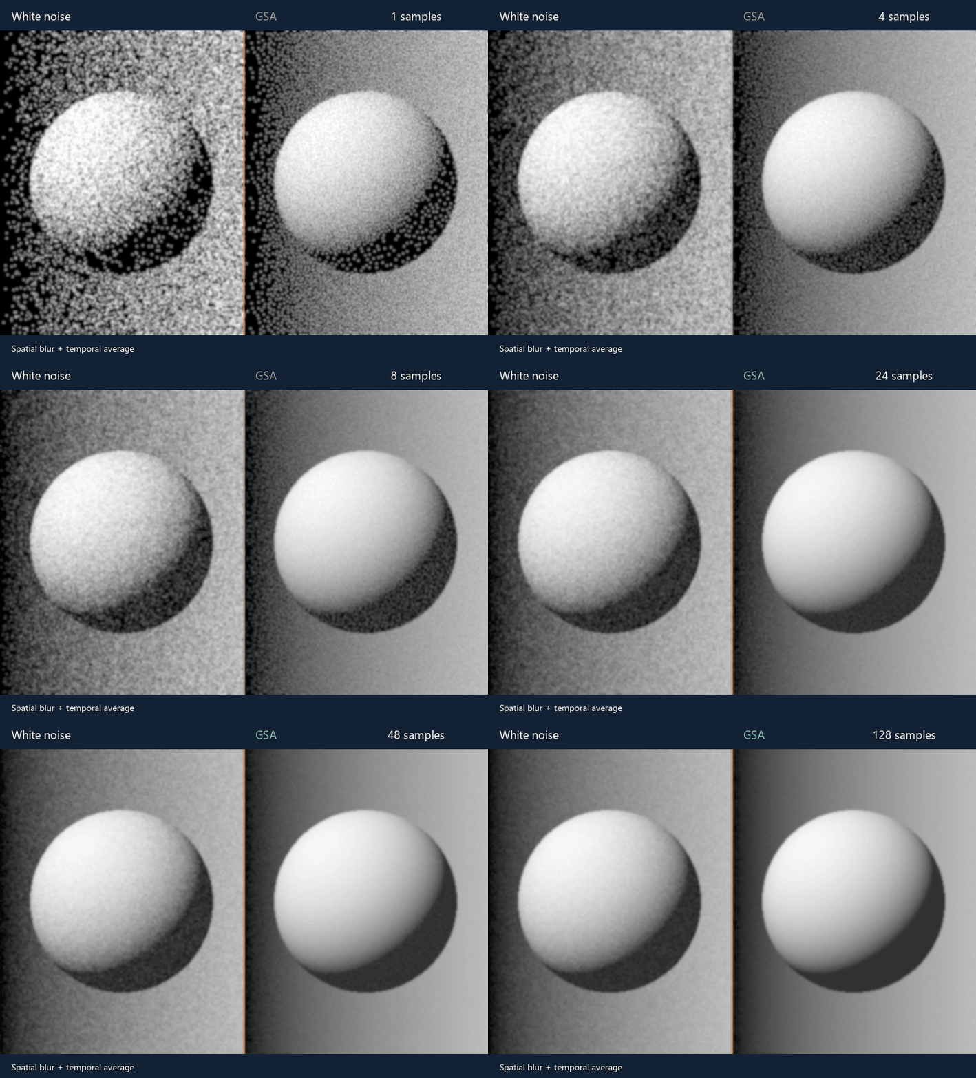
White noise is on the left; GSA is on the right. The Three.js example accumulates 1 to 128 samples with spatial and temporal filtering.
Blue noise is about the error after sampling#
A pleasing noise texture is not enough. A renderer transforms random numbers through some function: a visibility test, a sampling transform, a material response. What matters is the error after that transformation and after reconstruction.
Scalar Spatiotemporal Blue Noise Masks develops masks with useful spatial and temporal behavior. FAST, Filter-adapted Spatiotemporal Sampling, takes the filter and a class of integrands into account when constructing samples. Its implementation and textures are the foundation for GSA. Related screen-space sampler research also evaluates transformed sampling error after a spatial blur.
For a scalar test function , the basic quantity we measure is
Here is the sample at pixel and frame . We can inspect this error directly, spatially blur it, or replace the finite average with an exponential moving average. Different functions and filters expose different weaknesses.
This distinction became central to the search. An early cheap method made the average of the raw scalar samples exceptionally close to one half. It looked spectacular on the first chart, but performed badly after nonlinear transformations. Arranging cancellation for does not guarantee good samples for a threshold, let alone a renderer.
How GSA constructs the texture#
The current profile constructs a periodic volume: 32 scalar samples for each pixel in a spatial tile. It starts from a seed, without an existing optimized texture.
First, give every pixel a stratified temporal distribution. Split into 32 equal intervals. Draw one independently jittered value from each interval, then randomly permute those values across the 32 frames. Each pixel therefore begins with good full-cycle coverage of the scalar domain.
Then optimize the ordering while preserving those values. Proposed exchanges swap two temporal positions within the same pixel. The set of samples belonging to that pixel never changes. The optimizer can improve how neighboring pixels and nearby frames relate without destroying that pixel's full-cycle stratification or changing its full-cycle mean.
The sample-distance term is
The absolute-difference term retains FAST's continuous threshold-oriented objective. The additional squared-difference term gives raw-value integration error an explicit role. Keeping the threshold term matters: it prevents us from optimizing only the scalar cancellation that misled the initial screen.
The filter objective combines 80% of the original separate spatial/temporal kernel with 20% of a compact space-time product term, truncated to radius two along each axis. We checked the spectrum of the implemented Float32 combined kernel on 21 periodic grids: every eigenvalue was positive, with a minimum of approximately 0.138983 on the default grid. This validates the combined kernel for the checked configurations; changing its weights or dimensions requires another check.
Many candidate exchanges run in parallel on the GPU. A minimum suppression factor of two reduces interference between neighboring updates, although favorable individual exchange estimates still do not guarantee a globally decreasing objective when exchanges happen together.
Finally, annealing lets the optimizer escape a greedy local minimum. For the first 1,500 iterations, a Metropolis acceptance rule sometimes accepts an unfavorable exchange. Its temperature falls linearly from 0.001 to zero. Another 1,500 greedy iterations finish the volume. The comparable greedy constrained optimizer stalled; increasing its budget to 10,000 iterations produced exactly the same output as its 3,000-iteration run.
Neither stratification nor simulated annealing is a new invention. FAST already uses stratified initialization, describes its optimizer in terms of annealing, and discusses temperature-dependent acceptance schedules. Its initialization preserves each spatial slice's histogram; GSA instead preserves each pixel's temporal strata. GSA names this combination of constraints, loss, filter mixture and schedule, building on those established principles.
What the convergence chart shows#
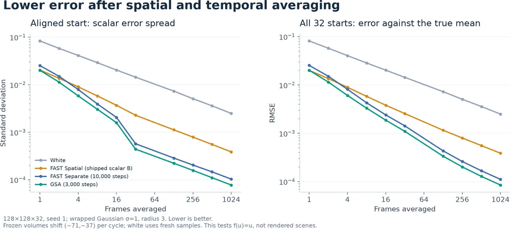
Lower error is better. The simple spread measurement reproduces the original scalar experiment. The phase-aware panel measures error against the known integral over all 32 temporal start phases, including the spatial shift used when the volume wraps.
The first experiment accumulated noise values and measured the remaining spread, with and without spatial blur, at increasing frame counts. GSA does well here because it combines good temporal coverage with an ordering optimized for reconstruction.
There is an important qualification at 32 frames. Starting at the beginning of a volume and averaging a complete cycle is especially favorable to the preserved temporal strata. A standard deviation measures variation across pixels; it does not include a uniform bias. A real consumer can also begin partway through a cycle, crossing the boundary where the tile shifts spatially.
We therefore also measure RMSE against the known integral over every temporal starting phase, with the actual playback convention. For the 32-frame, spatially blurred case, GSA reduces identity-function RMSE by about 23%, threshold-at-one-half RMSE by about 26%, square-function RMSE by about 20%, and fourth-power RMSE by about 15% on seed 1. These are more informative than presenting the largest aligned-cycle scalar improvement as a general convergence gain.
The results are real improvements for these measurements. Their size also reflects what the generator is designed to preserve and optimize.
A broader audit, including the losses#
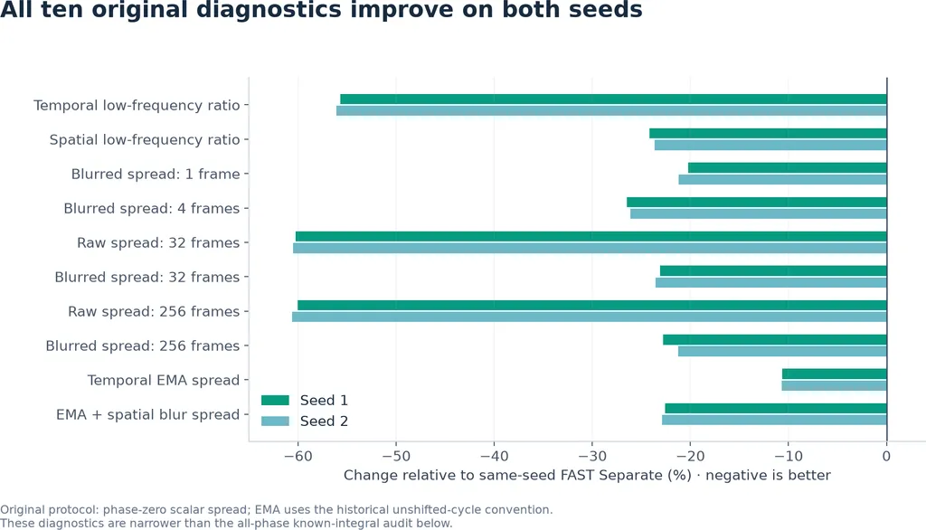
GSA divided by the matching FAST Separate reference; below one is better. All ten original measurements improve on both seeds. Each ratio compares the same measurement between samplers.
The original ten measurements cover spatial and temporal low-frequency power, raw temporal error, spatially blurred error at several frame counts, and exponential accumulation with and without blur. GSA improves all ten on both tested seeds.
That was encouraging, but the earlier false lead made a broader check essential. The expanded suite contains 318 diagnostics: the original ten plus 308 integration-error measurements. It evaluates 22 known-integral functions, raw and spatially blurred, at six finite accumulation lengths and one exponential accumulation setting. All textures are quantized to the same 8-bit bin centers before scoring.
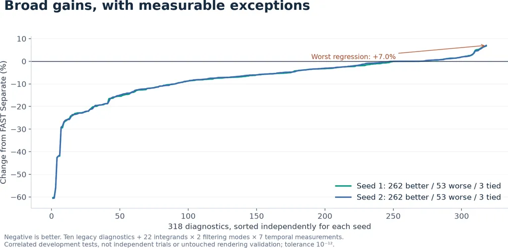
Each measurement compares GSA with a freshly generated, same-seed, 10,000-iteration FAST Separate reference. Negative error changes favor GSA.
On each of seeds 1 and 2, GSA wins 262 measurements, loses 53, and ties three, using an absolute tie tolerance of . The median relative error change on seed 1 is approximately 5.6% lower. Counting wins alone hides their magnitude, which is why the chart retains the regressions.
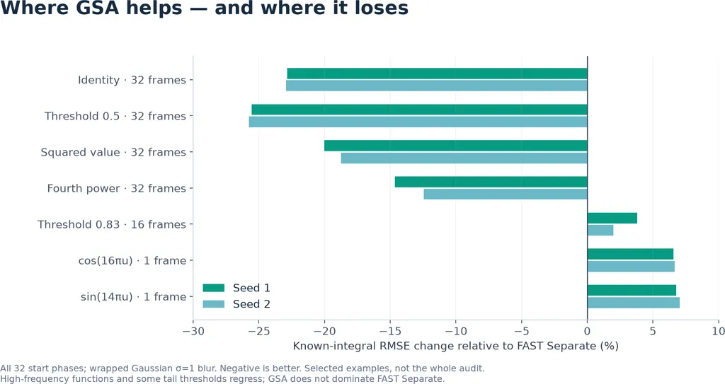
The stronger temporal and filtered results coexist with weaker high-frequency transformed-function cases. These are selected illustrations; the full audit remains available with the research code.
The worst losses are single-frame, spatially blurred high-frequency functions. For , error is about 6.77% higher on seed 1 and 7.03% higher on seed 2. For , it is about 6.55% and 6.66% higher. A threshold at 0.83 after 16 frames with spatial blur also regresses by roughly 3.8% on seed 1.
These results favor FAST when single-frame, high-frequency transformations dominate the workload.
Which rendering workloads benefit?#
We then evaluated six geometric workloads with analytic references, independently generated masks for sampling dimensions, two seed pairs, six frame counts, two temporal filters and three spatial filters. The 432 matched comparisons measure total RMSE against the current unfiltered truth, including reconstruction and temporal-history bias.
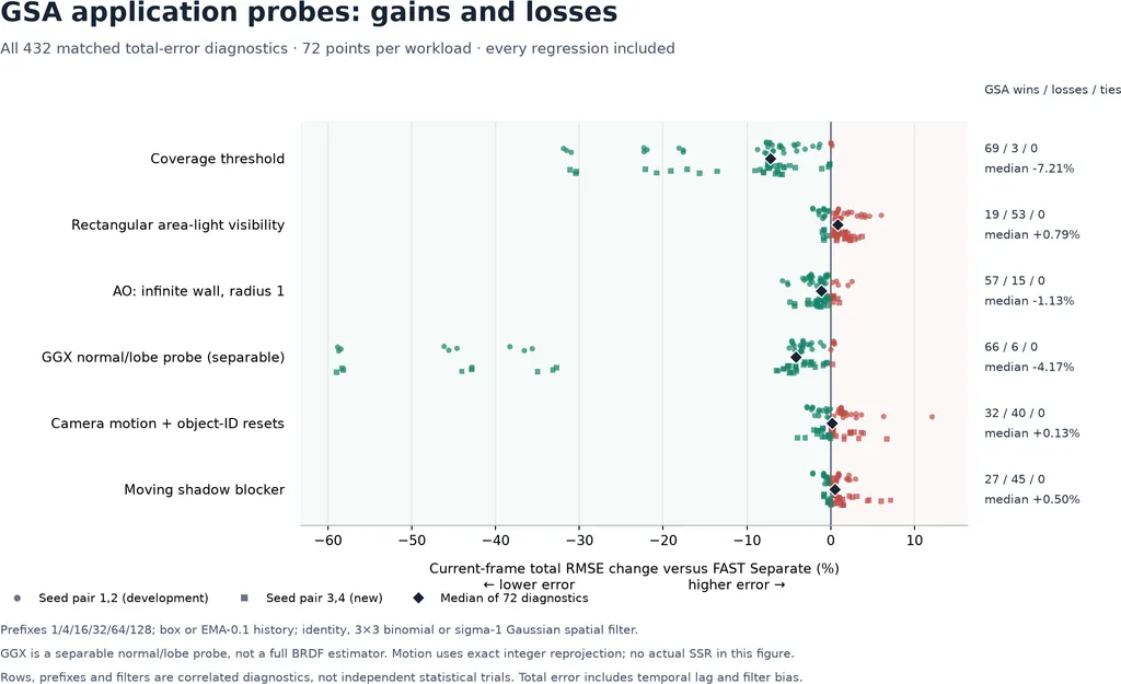
| Workload | Lower / higher error | Median error change |
|---|---|---|
| Stochastic coverage | 69 / 3 | −7.207% |
| GGX normal/environment lobe probe | 66 / 6 | −4.173% |
| Finite-distance AO with an infinite wall | 57 / 15 | −1.128% |
| Static rectangular-light shadow | 19 / 53 | +0.795% |
| Moving-blocker rectangular-light shadow | 27 / 45 | +0.496% |
| Camera/parallax shadow with history resets | 32 / 40 | +0.125% |
Negative changes favor GSA. Each row contains 72 filter/frame/seed-pair comparisons.
Across all six workloads, GSA lowers error in 270 comparisons and raises it in 162. The practical recommendation follows the individual rows: choose GSA for the tested coverage and AO workloads, and FAST for these rectangular-light shadows. The GGX probe evaluates a separable normal/environment lobe; the SSR test below evaluates coupled reflection sampling.
The camera test moves foreground and background at different rates, reprojects history using exact object motion, and resets history at newly revealed pixels and object-ID changes. Its near-neutral aggregate result shows why strong static accumulation alone is insufficient when choosing a sampler for moving content.
Returning to Three.js SSR#
The final test uses Three.js's actual stochastic SSRNode, with three metallic floor strips at roughness 0.12, 0.3 and 0.65, colored boxes and a fixed camera. It renders at 128×128 using WebGPU. Four independently generated scalar masks supply the sampling dimensions. A separate 4,096-sample PCG reference measures convergence to the same SSR algorithm.
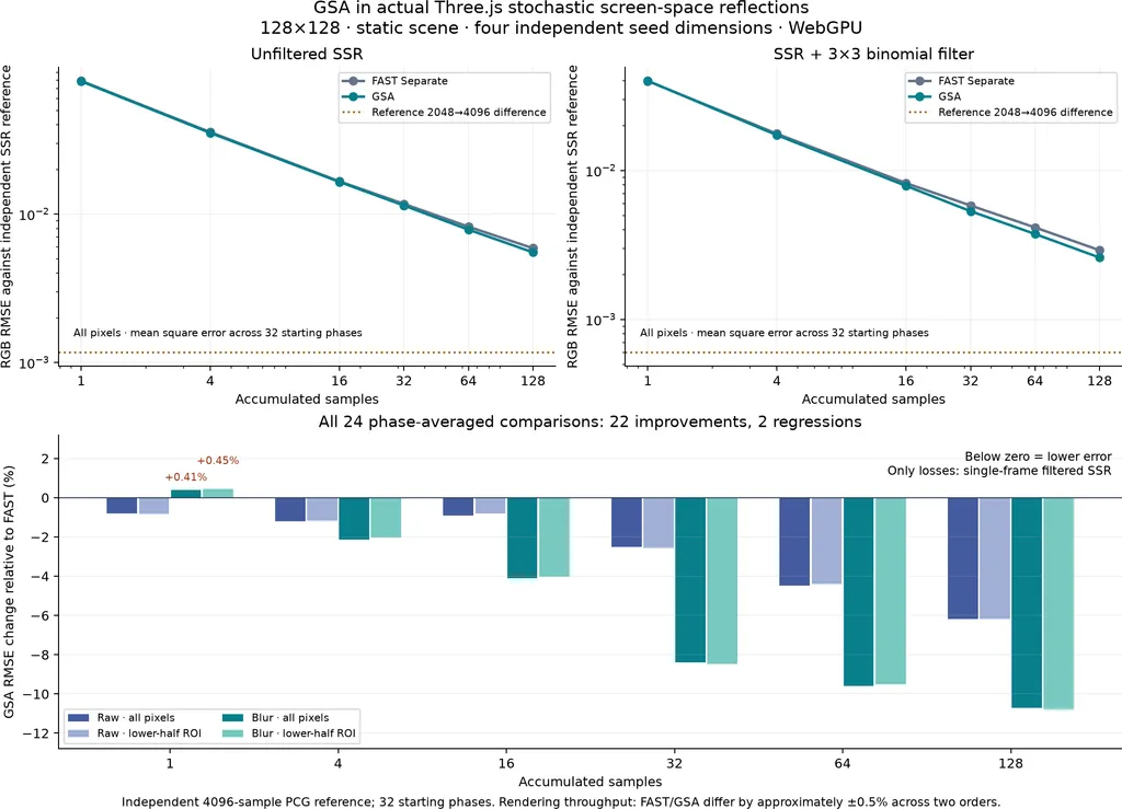
RMSE includes all 32 temporal starting phases. The chart reports raw output and identical 3×3 binomial filtering, for the full image and a fixed foreground-floor region.
GSA improves 22 of the 24 phase-averaged measurements. Full-image spatially filtered RMSE is 8.38% lower at 32 frames, 9.60% lower at 64 frames and 10.70% lower at 128 frames. At 64 and 128 frames, every starting phase improves with both filters. The two losses are one-frame blurred error: approximately 0.41% higher for the full image and 0.45% higher for the floor region.
This makes GSA a good choice for filtered accumulation in this static SSR workload. Rendering throughput is effectively unchanged between the two samplers, while GSA produces a cleaner accumulated image.
Offline construction and texture delivery#
The construction benchmark runs FAST Separate and GSA sequentially after warmup, completing generation and readback before starting the next run.
| Seed | FAST Separate, 10,000 iterations | GSA, 3,000 iterations | Speedup |
|---|---|---|---|
| 1 | 61.233 s | 30.720 s | 1.993× |
| 2 | 61.339 s | 30.756 s | 1.994× |
GSA's evaluated 3,000-iteration profile generates its mask about 2× faster than the 10,000-iteration FAST Separate reference. These end-to-end times include initialization, optimization and readback. The benchmark records contain the full configuration and timing details.
At roughly 31 seconds, generation is too slow for startup in a real-time application. The example loads a pregenerated scalar PNG of approximately 0.53 MB and caches it. The older roughly 3.03 MB FAST asset packs multiple sample distributions and channels; this example needs only the scalar mask. These assets contain different payloads, so their sizes do not establish a compression or download-size advantage for GSA. Precomputation still leaves a texture to distribute.
The standalone repository separates generation from consumption: generate assets offline, then load them at runtime. Its example provides filter controls and a side-by-side comparison for evaluating the sampler in your own pipeline.
After checking out the repository and installing its workspace dependencies, generation and Three.js texture creation use separate entry points:
import { generateGSA } from 'three-gsa/generator';
import { createGSADataTexture } from 'three-gsa/three';

const volume = await generateGSA(); // evaluated 128×128×32, 3,000-step defaults
const atlas = createGSADataTexture(volume);
// Use the library's playback helper; dispose atlas when finished.
Applications loading a pregenerated PNG can omit the optimizer entirely.
What the AI exploration contributed#
I used an AI-directed process to propose alternatives, implement them in parallel, and evaluate them against common references. The search covered hierarchical constructions, lattice sequences, local relaxation, threshold refinement, feature-based objectives, GPU constraints and annealing schedules. Most candidates were rejected or retained only as useful counterexamples.
The most valuable part was the cycle of implementation, numerical review and expanding the evaluation when a result looked suspiciously good. That exposed the raw-scalar cancellation artifact and led to transformed-function tests, bias-aware RMSE, phase-aware playback and a second seed.
The scalar diagnostics guided configuration selection. We then kept that configuration fixed while adding the geometric workloads, new seed pairs and the rendered SSR scene.
GSA is the result of that AI-guided exploration: a combination of established techniques that improves several measured workloads while leaving clear regressions. The geometric tests and native SSR scene show where the gains carry into rendering. The implementation, profiles and measurements are available to reproduce and extend the search.